How much will it cost to mitigate climate change?

United Nations (UN) member states signed the latest climate agreement, The Paris Agreement, in 2015; the agreement set an international target to limit average global warming to two degrees celsius above pre-industrial temperatures. An important question then arises: how do we achieve this, and how much will it cost to keep warming below the two degree target?

So, how do we estimate the economic cost of mitigating climate change? The most common way of measuring—and visualizing—the options and costs of reducing our greenhouse gas (GHG) emissions is to use the so-called ‘abatement cost curve’ (sometimes referred to as the ‘marginal abatement curve’). Here we will explore what these curves are and how we use them. But before proceeding, it’s important to note that these curves can be used at a range of levels to assess the best and most economic options we have for reducing GHG emissions. In particular, they can be constructed at global, regional, national or city levels. As such, a range of different abatement cost curves exist. In this post, we will be looking at a global curve developed by McKinsey & Company.¹ Although we could have looked at a number of different examples, this analysis in particular is one of the most widely-referenced and accepted to date.

Here is a preview of what these abatement costs tell us: If we aggressively pursue all of the low-cost abatement opportunities currently available, the total global economic cost would be €200-350 billion per year by 2030. This is less than one percent of the forecasted global GDP in 2030.

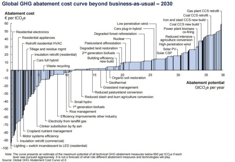
An abatement cost curve measures two key variables, as shown on McKinsey’s chart below: abatement potential and the cost of abatement.

‘Abatement potential’ is the term we use to describe the magnitude of potential GHG reductions which could be technologically and economically feasible to achieve. We measure this in tonnes of greenhouse gases (which is measured here as carbon dioxide equivalents, or CO₂e and which include all greenhouse gases, not just CO₂.² So, on the x-axis we have the abatement potential of our range of options for reducing our GHG emissions; here, each bar represents a specific technology or practice.³ The wider the bar, the greater its potential for reducing emissions.

On the y-axis we have the abatement cost. This measures the cost of reducing our GHG emissions by one tonne by the year 2030, and in this case is given € per tonne of CO₂e saved.⁴ But it’s important to clarify here what we mean by the term ‘cost’. ‘Cost’ refers to the economic impact (which can be a loss or gain) of investing in a new technology rather than continuing with ‘business-as-usual’ technologies or policies. To do this, we first have to assume a ‘baseline’ of what we expect ‘business-as-usual’ policies and investments would be. This is done—for both costs and abatement potential—based on a combination of empirical evidence, energy models, and expert opinion.⁵ This can, of course, be challenging to do; the need to make long-term predictions/projections in this case is an important disadvantage to cost-abatement curves. Whilst not perfect, it does provide useful estimates of relative costs and abatement potential.

Let’s use an example to explain these costs. The majority of the world’s private vehicles are currently diesel or gasoline-powered. Our baseline or ‘business-as-usual’ scenario in this case would be that everyone continues driving vehicles run on fossil fuels, and that growth in the car market continues in line with market projections through to 2030. One option we might consider to reduce CO₂ is to begin replacing these with electric-powered vehicles. Electric vehicles (at least currently) are typically more expensive than similar gasoline-powered vehicles, so buying an electric vehicle would require a notably higher investment than ‘business-as-usual’. However, with time, the running or operating costs of an electric vehicle may be lower than a traditional car (as a result of efficiency gains and lower cost of electricity relative to liquid fuel), so we will begin to get some economic return on our initial investment. This scenario—in which we need an up-front investment in new technology—typically means that the capital intensity of the opportunity is high; but spread across years of operation, the annual average cost falls.

Our potential mitigation options are ordered from left-to-right in terms of cost (getting progressively more expensive as we move to the right). The higher the bar, the greater the cost. McKinsey’s analysis defines an upper cost threshold of €60 per tonne avoided (i.e. the chart only shows alternatives that are ‘cheaper’ than €60 per tonne). This is the level they consider to be most economically attractive to investors. This figure is somewhat arbitrary, and as we will see later, the report has also estimated potential emissions savings from technologies above €60 per tonne separately.

As you see many options to the left-hand side of the curve have negative costs. Negative costs indicate options which would actually save money. These are typically related to energy efficiency or land management projects which would provide an economic return over the longer-term.

For example, replacing conventional lighting with energy efficient lighting, would more than pay back in economic terms from lower energy bills. Its ‘cost’ is therefore negative because we would actually save money. Globally, if we took advantage of all of our negative cost options, we see that we could cumulatively avoid emissions of 11-12 billion tonnes of CO₂e.

At the other end of the scale we have the more expensive options for mitigation; these are typically related to the supply with low-carbon energy from solar, wind, nuclear, and carbon capture and storage (CCS).

Abatement cost curves are used at a range of scales to aid investment decisions on GHG mitigation options. When making these decisions, both the abatement potential (width) and cost (height) of each option is important. For example, if we look at the lowest end of the scale we see that installing energy efficient lighting is the most cost-effective option (providing a high economic return through efficiency savings). However, its total abatement potential is small. If we were looking for an investment which could save a large quantity of GHGs, we might have to select an option which is more expensive, but has a greater abatement potential. The trade-off between cost and potential is an important one.

Global greenhouse gas abatement cost curve⁶

If we were to implement all of our options for reducing GHG emissions, how much CO₂e would we save?

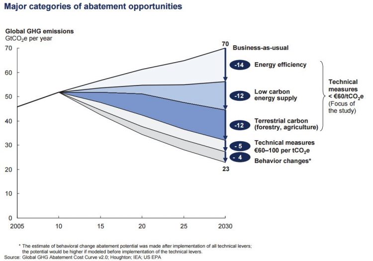
On the abatement cost curve above we see that cumulatively, the options costing up to €60 per tonne have a total abatement potential of 38 billion tonnes of CO₂e per year (this is the total width along the horizontal axis). This total potential has been summarized in the chart below. On the y-axis we have our global GHG emissions in billion tonnes of CO₂e, and on the x-axis we see this evolution with time through to 2030.

The top line we see in this chart is our ‘business-as-usual’ (BAU) pathway. This is our projection of how global emissions would increase if we don’t invest in technology and practices necessary to reduce emissions; this pathway is calculated based on expected population and economic growth projections. By 2030, with business-as-usual, we would expect our annual emissions to be 70 billion tonnes CO₂e.

Below this line, we see our options for reducing emissions. Our <€60 per tonne abatement opportunities have been decomposed into energy efficiency, low-carbon energy supply and terrestrial carbon (forestry and agriculture) options. Combined, these would mean that we avoid 38 billion tonnes of emissions.

But we also have two additional opportunities where we could make GHG savings. The first lies in more expensive technical measures, costing €60-100 per tonne avoided. Such opportunities are not unattainable, however, we might expect the range of cheaper options to have a significantly greater uptake before more expensive technologies are adopted. The second additional opportunity lies in social and behavioral changes which influence energy consumption and consumer choices towards lower-carbon options.

If we include these additional opportunities, our maximum technical abatement potential by 2030 totals 47 billion tonnes of CO₂e per year. Our maximum global potential is therefore a 65-70% reduction relative to our current projected pathway.

Global greenhouse gas abatement potential⁷

How much would it cost in total to implement all of these options?

We can calculate this value using our abatement cost curve. The area of each of our bars represents the total cost for each technology or strategy. By adding all of these individual costs, we get the total economic cost. To get the approximated annual cost, we can divide this total by the number of years until our target date (in this case, the year 2030). This method is not strictly accurate, since it assumes that costs will be distributed equally across this timeframe; however, it gives us some relative approximation.

If we utilized all of our <€60 per tonne abatement opportunities to their full potential (which is an important assumption), McKinsey estimates the total global cost to be €200-350 billion per year by 2030. This is less than one percent of the forecasted global GDP in 2030.

This cost is however, made more complex by the timing of investment. This timing component is important for financing and capital investment. Our average annual cost is calculated as a balance of how much money we need to invest, and how much we get in return based on efficiency gains and reduced running costs relative to our current technologies. However, as we noted earlier, we often need an initial capital invesment to implement the technology; this initial capital can be high, but begins to pay back over time (resulting in a reduction in the average annual cost through time). The upfront capital investment needed is €530 billion per year by 2020 and €810 billion by 2030. Although these figures may seem substantial, many estimates project that the economic costs of not taking action to avert climate change would greatly exceed investments in mitigation opportunities.⁸

Technical notes:

It should be noted that the figures presented in cost abatement curves carry significant uncertainty and interdependencies. The total abatement cost curve is developed based on the construction and combination of individual bars related to a particular technology or practice. The width and height (i.e. abatement potential and cost) is measured independently of other technologies and variables on the curve. However, this assumption is a large and important one: many technologies (for example, solar PV and battery storage) have strong interdependencies. The evolution of one will inevitably have some impact on the other.

Technology costing is also strongly dependent on scaling effects–unit costs often decrease as capacity increases. The individual costs represented on these charts are therefore calculated with the assumption that the development and scale-up of the respective technology is approached aggressively and full technical potential is achieved. Changes in technology prices through time are assumed based on technology-specific ‘learning curves’. Learning curves measure the reduction in cost for every doubling in a technology’s capacity. For example, the learning rate for solar PV has been 22% –this means that the cost per unit of power falls by 22% for every doubling of capacity.⁹ This analysis assumes that the learning rate for specific technologies remains consistent with past trends.

McKinsey&Company stress that their estimates therefore carry a high level of uncertainty. They are useful in providing an overview outlook on the total abatement potential (and whether this would be sufficient to meet global climate targets) and estimate the potential costs of doing so. Their most useful function is perhaps in allowing for relative comparisons of costs and potential between different technologies; these factors are key for decision-makers looking to investment in low-carbon opportunities. Although imperfect, they give a relative sense of magnitude of what could potentially be achieved and if the costs can be managed to do so.